41 row labels in excel pivot table
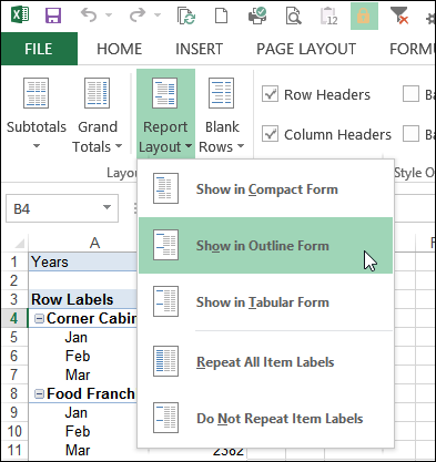
Microsoft Excel - showing field names as headings rather ... In earlier versions, by default if you create a pivot table, instead of showing the field names, it will say row labels and column labels. To see the field names instead, click on the Pivot Table Tools Design tab, then in the Layout group, click the Report Layout dropdown and select either Show in Outline Form or Show in Tabular form. How to unbold Pivot Table row labels - MrExcel Message Board Using Excel 2007, nested Pivot Table rows always seem to bold all but the inner-most row label. Is there a way to unbold all row labels? Displaying in Classic layout, tabular form, without expand/collapse buttons. Showing/Hiding subtotals doesn't seem to matter. I don't recall older versions...
How to Customize Your Excel Pivot Chart Data Labels - dummies The Data Labels command on the Design tab's Add Chart Element menu in Excel allows you to label data markers with values from your pivot table. When you click the command button, Excel displays a menu with commands corresponding to locations for the data labels: None, Center, Left, Right, Above, and Below.

Row labels in excel pivot table
Use column labels from an Excel table as the rows in a ... Close the dialog and keep the changes. Excel should place the unpivoted data into a new worksheet, looking something like this: Now the final step is to create a pivot table using this unpivoted data. Here is a screenshot of my pivot table setup: Note that Attribute (e.g. Malaria, Tuberculosis) is placed above the Year. This lets us open or ... Pivot table row labels in separate columns • AuditExcel.co.za So when you click in the Pivot Table and click on the DESIGN tab one of the options is the Report Layout. Click on this and change it to Tabular form. Your pivot table report will now look like the bottom picture and will be easier to use in other areas of the spreadsheet and in our opinion is also easier to read. excel - Custom row labels in PivotTable - Stack Overflow 1 you can give nicknames to the fields that you are checking which populate the pivot table. If you go the pivot table data and right click you can change the value field settings to give a custom name to a row/series but I do not know about individual data points. path: pivot table data => right click => select Field Settings => edit custom name.
Row labels in excel pivot table. Gallery of 33 pivot table blank row label labels database ... 33 Pivot Table Blank Row Label Labels Database 2020 images that posted in this website was uploaded by Film.norden.org. 33 Pivot Table Blank Row Label Labels Database 2020 equipped with a HD resolution 687 x 377.You can save 33 Pivot Table Blank Row Label Labels Database 2020 for free to your devices. get a row label from pivot table - Microsoft Tech Community Re: get a row label from pivot table @omdl2020 That's how GETPIVOTDATA works. If you don't want that, it's better to use SUMIFS based on the source data. Enter A and B in M3 and M4. How to Add Rows to a Pivot Table: 9 Steps (with Pictures) Click Add under "Rows." It's in the left side of the pivot table editor. A list of fields will expand on the menu. 4 Click the name of the field you want to add as a row. Rows are usually non-numeric fields, such as category names and/or column headers. Once you select a field, a new row or rows will be added for the items in that field. How to Use Excel Pivot Table Label Filters You can use a similar technique to hide most of the items in the Row Labels or Column Labels. Select the pivot table items that you want to keep visible Right-click on one of the selected items In the pop-up menu, click Filter, then click Keep Only Selected Items. All but the selected items are immediately hidden in the pivot table.
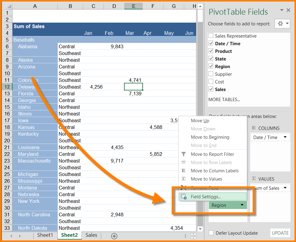
Excel 2016 Pivot table Row and Column Labels - Microsoft ... In Excel 2016 I've found when I create a pivot table it unhelpfully shows 'Row Labels' and 'Column Labels' instead of my field names, although in the top left cell it says 'Count of' and then inserts the correct field name. Years ago when I last used Excel it automatically put the field names in all three heading cells. How to make row labels on same line in pivot table? Make row labels on same line with PivotTable Options You can also go to the PivotTable Options dialog box to set an option to finish this operation. 1. Click any one cell in the pivot table, and right click to choose PivotTable Options, see screenshot: 2. PivotTable Count of Row Labels - Excel Help Forum Re: PivotTable Count of Row Labels. Please choose "Index" Option under the Pivot Table field options. Right Click on the field - "Value Field Settings" - "Show Value As" - chose "Index". Register To Reply. 05-15-2014, 12:17 PM #8. Repeat item labels in a PivotTable Right-click the row or column label you want to repeat, and click Field Settings. Click the Layout & Print tab, and check the Repeat item labels box. Make sure Show item labels in tabular form is selected. Notes: When you edit any of the repeated labels, the changes you make are applied to all other cells with the same label.
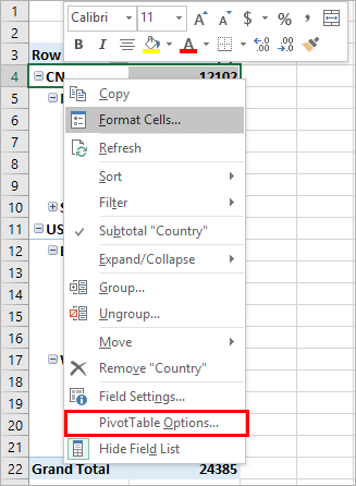
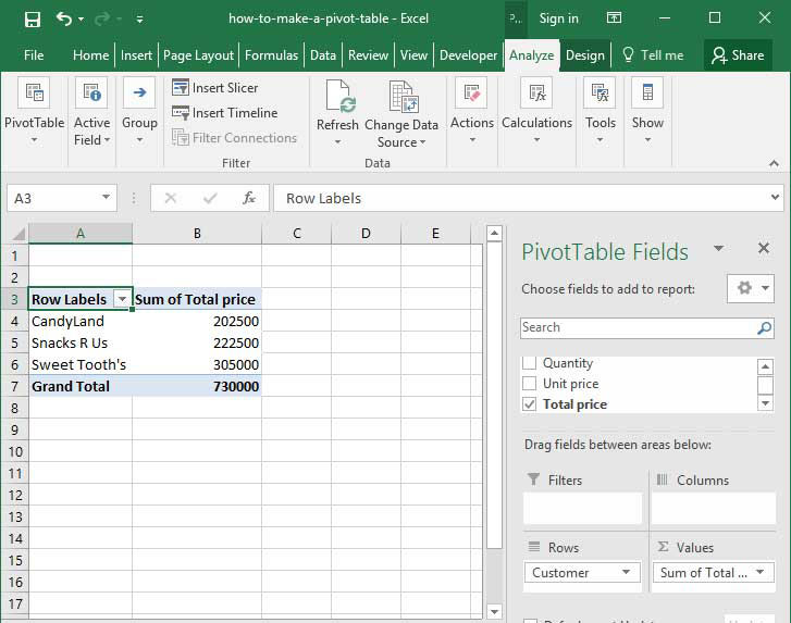
How to rename group or row labels in Excel PivotTable? To rename Row Labels, you need to go to the Active Field textbox. 1. Click at the PivotTable, then click Analyze tab and go to the Active Field textbox. 2. Now in the Active Field textbox, the active field name is displayed, you can change it in the textbox. Changing Blank Row Labels - Excel Pivot Tables Select one of the Row or Column Labels that contains the text (blank). Type N/A in the cell, and then press the Enter key. Note: All other (Blank) items in that field will change to display the same text, N/A in this example. For more information on pivot tables, see the Pivot Table Topics on my Contextures web site. Change the pivot table "Row Labels" text | MrExcel Message ... Feb 4, 2021. #3. mart37 said: Click on the cell and typ the text. Click to expand... Thanks mart37. So simple! I was looking for a way to change it on the ribbons & settings. Typical Excel - things you think are difficult are easy, and things that should be easy are difficult! Design the layout and format of a PivotTable Click anywhere in the PivotTable. This displays the PivotTable Tools tab on the ribbon. On the Options tab, in the PivotTable group, click Options. In the PivotTable Options dialog box, click the Layout & Format tab, and then under Layout, select or clear the Merge and center cells with labels check box.

Pivot table row labels in separate columns • AuditExcel.co.za
Microsoft Excel - showing field names as headings rather ... In Microsoft Excel 2007 and 2010, by default if you create a pivot table, instead of showing the field names, it will say row labels and column labels. Show in Outline Form or Show in Tabular form. The relevant labels will
How to Create Pivot Tables in Microsoft Excel
Remove row labels from pivot table - AuditExcel.co.za Click on the Pivot table. Click on the Design tab. Click on the report layout button. Choose either the Outline Format or the Tabular format. If you like the Compact Form but want to remove 'row labels' from the Pivot Table you can also achieve it by. Clicking on the Pivot Table. Clicking on the Analyse tab.

Excel For Mac Pivot Table Repeat Item Labels - foxprofit
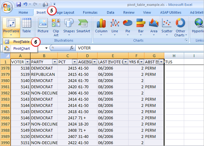
Automatic Row And Column Pivot Table Labels - How To Excel ... The first thing to do is put your cursor somewhere in your data list Select the Insert Tab Hit Pivot Table icon Next select Pivot Table option Select a table or range option Select to put your Table on a New Worksheet or on the current one, for this tutorial select the first option Click Ok
Advanced Excel | The Talk Buzz Forums
Pivot table row labels side by side - Excel Tutorials You can copy the following table and paste it into your worksheet as Match Destination Formatting. Now, let's create a pivot table ( Insert >> Tables >> Pivot Table) and check all the values in Pivot Table Fields. Fields should look like this. Right-click inside a pivot table and choose PivotTable Options…. Check data as shown on the image below.

How to Sort Pivot Table Row Labels, Column Field Labels and Data Values with Excel VBA Macro ...
Pivot Table "Row Labels" Header Frustration - Microsoft ... Hi Everyone please help I can't change my headers from Row Labels in a Pivot Table. Using Excel 365
How to make row labels on same line in pivot table?
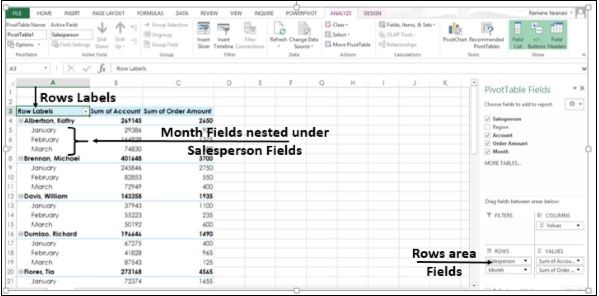
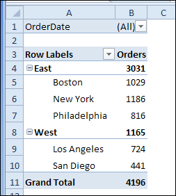
Move Row Labels in Pivot Table - Excel Pivot Tables Move Row Labels in Pivot Table When you add fields to the row labels area in a pivot table, the field's items are automatically sorted. See how you can manually move those labels, to put them in a different order. There's a video and written steps below. In the screen shot below, the districts are listed alphabetically, from Central to West.
In Search of the Elusive Pivot Table | Dynamic Edge, Inc. | Beyond Tech Support Dynamic Edge ...
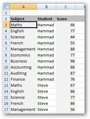
Multiple row labels on one row in Pivot table | MrExcel ... In Excel 2003, a pivot table would allow you to place multiple row labels on the left hand side of a pivot table. I can't figure out how to make that happen in Excel 2010. I need material and material description on the lefthand side of the pivot table but it is placing the description underneath on a 2nd row form the material number.

How to Sort Pivot Table Row Labels, Column Field Labels and Data Values with Excel VBA Macro ...
How to repeat row labels for group in pivot table? Except repeating the row labels for the entire pivot table, you can also apply the feature to a specific field in the pivot table only. 1. Firstly, you need to expand the row labels as outline form as above steps shows, and click one row label which you want to repeat in your pivot table. 2.
How To Make A Pivot Table | Deskbright
Pivot Table Row Labels In the Same Line - Beat Excel! First make a pivot table with required fields. Arrange the fields as shown in left picture. Your initial table will look like right picture. Now click on "Error Code" and access field settings. First check "None" option in "Subtotals & Filters" tab to disable totals after every row.
Repeat Pivot Table Labels in Excel 2010 – Excel Pivot Tables
excel - Custom row labels in PivotTable - Stack Overflow 1 you can give nicknames to the fields that you are checking which populate the pivot table. If you go the pivot table data and right click you can change the value field settings to give a custom name to a row/series but I do not know about individual data points. path: pivot table data => right click => select Field Settings => edit custom name.

excel - Extract Pivot Table Row Label (not value) - Stack Overflow
Pivot table row labels in separate columns • AuditExcel.co.za So when you click in the Pivot Table and click on the DESIGN tab one of the options is the Report Layout. Click on this and change it to Tabular form. Your pivot table report will now look like the bottom picture and will be easier to use in other areas of the spreadsheet and in our opinion is also easier to read.
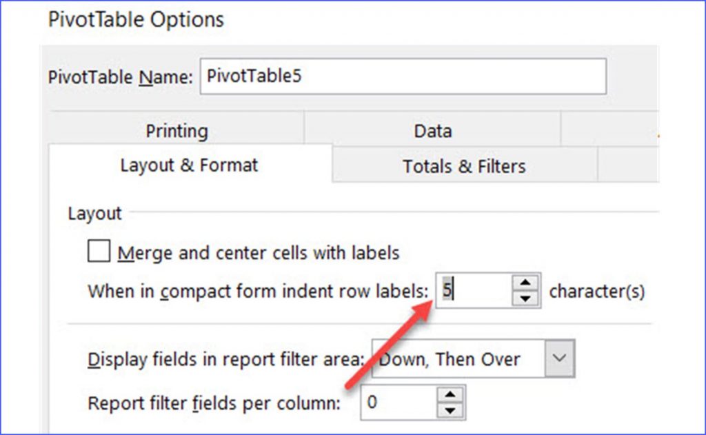
How to Increase Indent Row Labels in Pivot Table Compact Form - ExcelNotes
Use column labels from an Excel table as the rows in a ... Close the dialog and keep the changes. Excel should place the unpivoted data into a new worksheet, looking something like this: Now the final step is to create a pivot table using this unpivoted data. Here is a screenshot of my pivot table setup: Note that Attribute (e.g. Malaria, Tuberculosis) is placed above the Year. This lets us open or ...

How to make row labels on same line in pivot table?
Change Pivot Table to Outline Layout With VBA - Excel Pivot TablesExcel Pivot Tables
Excel - Mixed Pivot Table Layout | SkillForge
Post a Comment for "41 row labels in excel pivot table"